
PROJECT DETAILS
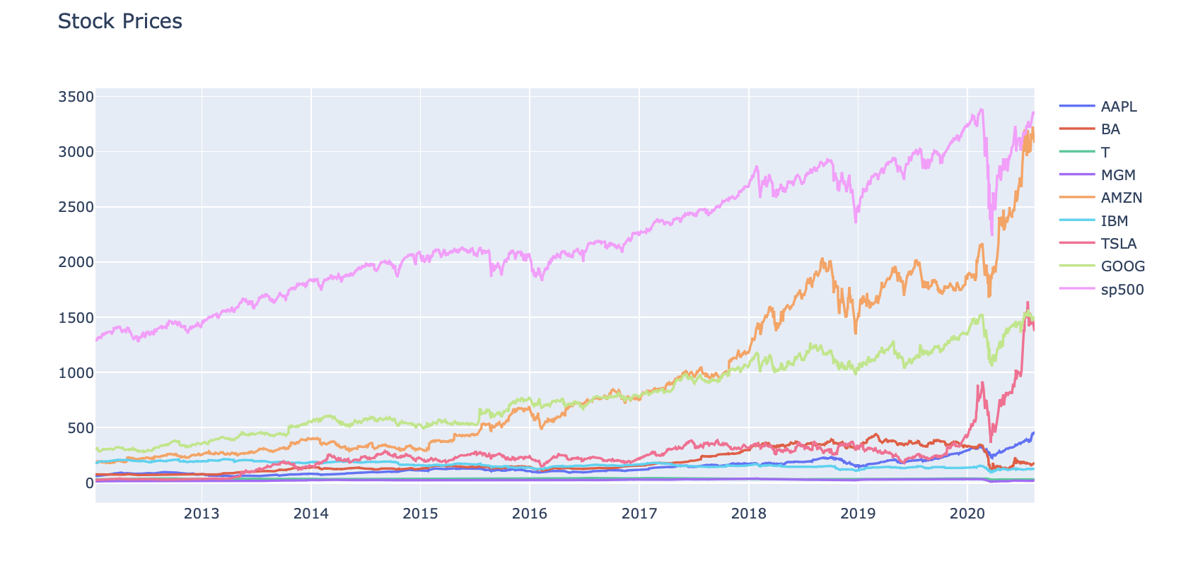
This project is on stock trading, specifically the SP500 & some very in demand stocks such as Apple, Amazon, and Google. The script will show the path that I took in order to get the most from the dataset visually and then explore a model that I found that could predict Apple’s stock to 92% accuracy. I then used the same model to the SP500 to show the ability to an index by using an LSTM model in keras. I hope you enjoy it and check out the code at my Github with the button above or share it with your network on Linkedin!
Math (Skip if you only want to see the fun stuff)
Ridge Regression is a way to create a model, when the number of predicator variables exceed the number of observations, or when the dataset has multicollinearity 🔔 (correlations between predictor variables). Also, the Ridge Regression is a L2 regression which add a penalty. The penalty is equal to the squares of the magnitude of coefficients. Penalty = Losing Money
So it is a perfect fit!
LSTM & Time Series LSTM is a recurrent neural network (RNN) that is trained by using Backpropagation through time and overcomes the vanishing gradient problem.
Long-Strong-Term Memory (LSTM) is the next generation of Recurrent Neural Network (RNN) used in deep learning for its optimized architecture to easily capture the pattern in sequential data aka STOCKS
🍻
Cheers! Now lets begin!!
IMPORT DATASETS AND LIBRARIES
# Data Maniupulation
import pandas as pd
import matplotlib.pyplot as plt
import numpy as np

# Data Visualization
import plotly.figure_factory as ff
import plotly.express as px

# Modeling
from sklearn.preprocessing import MinMaxScaler
from sklearn.linear_model import LinearRegression
from sklearn.model_selection import train_test_split
from sklearn.linear_model import Ridge
from tensorflow import keras

# Additional
from copy import copy
from scipy import stats
# Stock prices data
stocks_df = pd.read_csv('/Users/andrewdarmond/Documents/FinanceML/stock.csv')

# Stocks volume data
stocks_vol_df = pd.read_csv('/Users/andrewdarmond/Documents/FinanceML/stock_volume.csv')
# Sort the data based on Date
stocks_df = stocks_df.sort_values('Date')
# Sort the volume data based on Date
stocks_vol_df = stocks_vol_df.sort_values('Date')
PERFORM EXPLORATORY DATA ANALYSIS AND VISUALIZATION
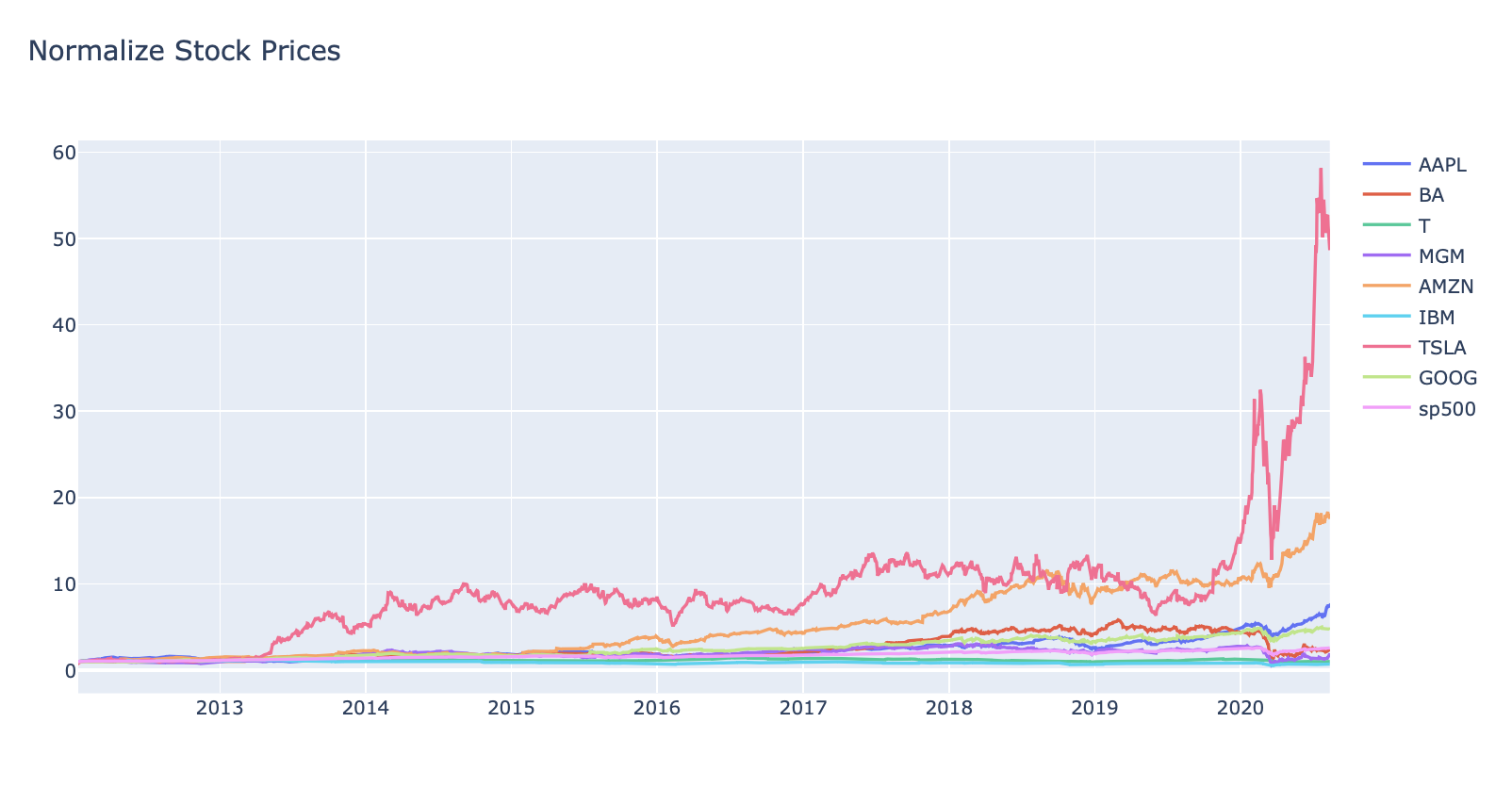
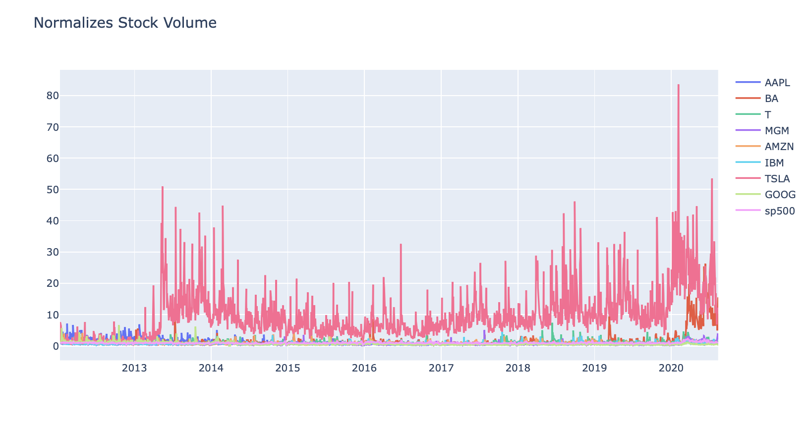
# Function to normalize stock prices based on their initial price
def normalize(df):
  x = df.copy()
  for i in x.columns[1:]:
    x[i] = x[i]/x[i][0]
  return x
# Function to plot interactive plots using Plotly Express
def interactive_plot(df, title):
  fig = px.line(title = title)
  for i in df.columns[1:]:
    fig.add_scatter(x = df['Date'], y = df[i], name =i)
  fig.show()
# plot interactive chart for stocks data
#interactive_plot(stocks_df, 'Stock Prices')
#interactive_plot(normalize(stocks_df), 'Normalize Stock Prices')
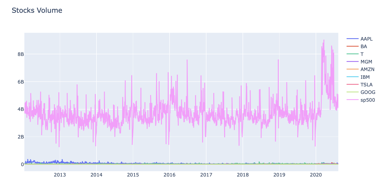
#interactive_plot(stocks_vol_df, 'Stocks Volume')
#interactive_plot(normalize(stocks_vol_df), 'Normalizes Stock Volume')
PREPARE THE DATA BEFORE TRAINING THE MODEL
# Function to concatenate the date, stock price, and volume in one dataframe
def individual_stock(price_df, vol_df, name):
  return pd.DataFrame({'Date': price_df['Date'], 'Close': price_df[name], 'Volume': vol_df[name]})
# Function to return the input/output (target) data for model
# Note that our goal is to predict the future stock price
# Target stock price today will be tomorrow's price
def trading_window(data):
  n = 1
  data['Target'] = data[['Close']].shift(-n)
  return data
If you want to view SP 500 / AMZN / ETC: Change ‘APPL’ HERE!
# Let's test the functions and get individual stock prices and volumes for AAPL
price_volume_df = individual_stock(stocks_df, stocks_vol_df, 'AAPL')
price_volume_df
| Date | Close | Volume | |
|---|---|---|---|
| 0 | 2012-01-12 | 60.198570 | 53146800 |
| 1 | 2012-01-13 | 59.972858 | 56505400 |
| 2 | 2012-01-17 | 60.671429 | 60724300 |
| 3 | 2012-01-18 | 61.301430 | 69197800 |
| 4 | 2012-01-19 | 61.107143 | 65434600 |
| ... | ... | ... | ... |
| 2154 | 2020-08-05 | 440.250000 | 30498000 |
| 2155 | 2020-08-06 | 455.609985 | 50607200 |
| 2156 | 2020-08-07 | 444.450012 | 49453300 |
| 2157 | 2020-08-10 | 450.910004 | 53100900 |
| 2158 | 2020-08-11 | 437.500000 | 46871100 |
2159 rows × 3 columns
price_volume_target_df = trading_window(price_volume_df)
price_volume_target_df
| Date | Close | Volume | Target | |
|---|---|---|---|---|
| 0 | 2012-01-12 | 60.198570 | 53146800 | 59.972858 |
| 1 | 2012-01-13 | 59.972858 | 56505400 | 60.671429 |
| 2 | 2012-01-17 | 60.671429 | 60724300 | 61.301430 |
| 3 | 2012-01-18 | 61.301430 | 69197800 | 61.107143 |
| 4 | 2012-01-19 | 61.107143 | 65434600 | 60.042858 |
| ... | ... | ... | ... | ... |
| 2154 | 2020-08-05 | 440.250000 | 30498000 | 455.609985 |
| 2155 | 2020-08-06 | 455.609985 | 50607200 | 444.450012 |
| 2156 | 2020-08-07 | 444.450012 | 49453300 | 450.910004 |
| 2157 | 2020-08-10 | 450.910004 | 53100900 | 437.500000 |
| 2158 | 2020-08-11 | 437.500000 | 46871100 | NaN |
2159 rows × 4 columns
# Remove the last row as it will be a null value
price_volume_target_df = price_volume_target_df[:-1]
price_volume_target_df
| Date | Close | Volume | Target | |
|---|---|---|---|---|
| 0 | 2012-01-12 | 60.198570 | 53146800 | 59.972858 |
| 1 | 2012-01-13 | 59.972858 | 56505400 | 60.671429 |
| 2 | 2012-01-17 | 60.671429 | 60724300 | 61.301430 |
| 3 | 2012-01-18 | 61.301430 | 69197800 | 61.107143 |
| 4 | 2012-01-19 | 61.107143 | 65434600 | 60.042858 |
| ... | ... | ... | ... | ... |
| 2153 | 2020-08-04 | 438.660004 | 43267900 | 440.250000 |
| 2154 | 2020-08-05 | 440.250000 | 30498000 | 455.609985 |
| 2155 | 2020-08-06 | 455.609985 | 50607200 | 444.450012 |
| 2156 | 2020-08-07 | 444.450012 | 49453300 | 450.910004 |
| 2157 | 2020-08-10 | 450.910004 | 53100900 | 437.500000 |
2158 rows × 4 columns
# Scale the data
sc = MinMaxScaler(feature_range = (0,1))
price_volume_target_scaled_df = sc.fit_transform(price_volume_target_df.drop(columns = ['Date']))
# Create Feature and Target
X = price_volume_target_scaled_df[:, :2]
y = price_volume_target_scaled_df[:, 2:]
price_volume_target_scaled_df.shape
(2158, 3)
X.shape, y.shape
((2158, 2), (2158, 1))
Spliting the data this way, since order is important in time-series
Note that we did not use train test split with it’s default settings since it shuffles the data
split = int(0.75 * len(X))
X_train = X[:split]
y_train = y[:split]
X_test = X[split:]
y_test = y[split:]
X_train.shape, y_train.shape
((1618, 2), (1618, 1))
X_test.shape, y_test.shape
((540, 2), (540, 1))
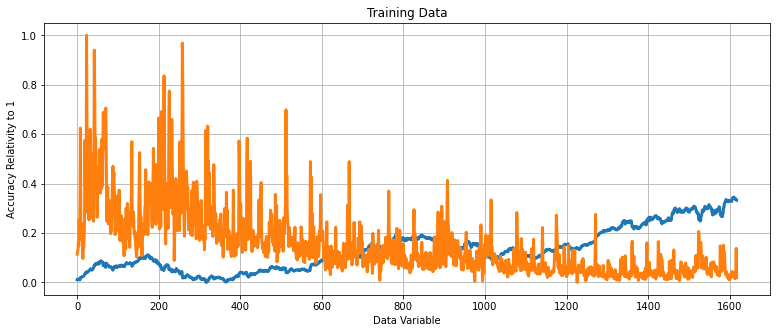
# Define a data plotting function
print('''
APPLE
''')
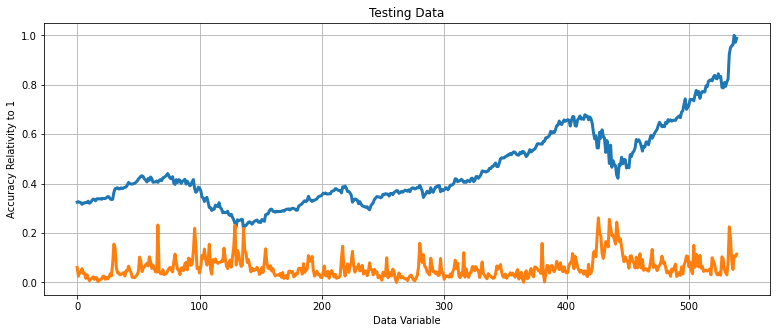
def show_plot(data, title):
plt.figure(figsize = (13, 5))
plt.plot(data, linewidth = 3)
plt.title(title)
plt.xlabel(xlabel= 'Data Variable')
plt.ylabel(ylabel= 'Accuracy Relativity to 1' )
plt.grid()
show_plot(X_train, 'Training Data')
show_plot(X_test, 'Testing Data')
APPLE
BUILD AND TRAIN A RIDGE LINEAR REGRESSION MODEL
regression_model = Ridge()

# Test the model and calculate its accuracy
regression_model.fit(X_train, y_train)

# Make Prediction
lr_accuracy = regression_model.score(X_test, y_test)
print('Ridge Regression Score:', lr_accuracy)
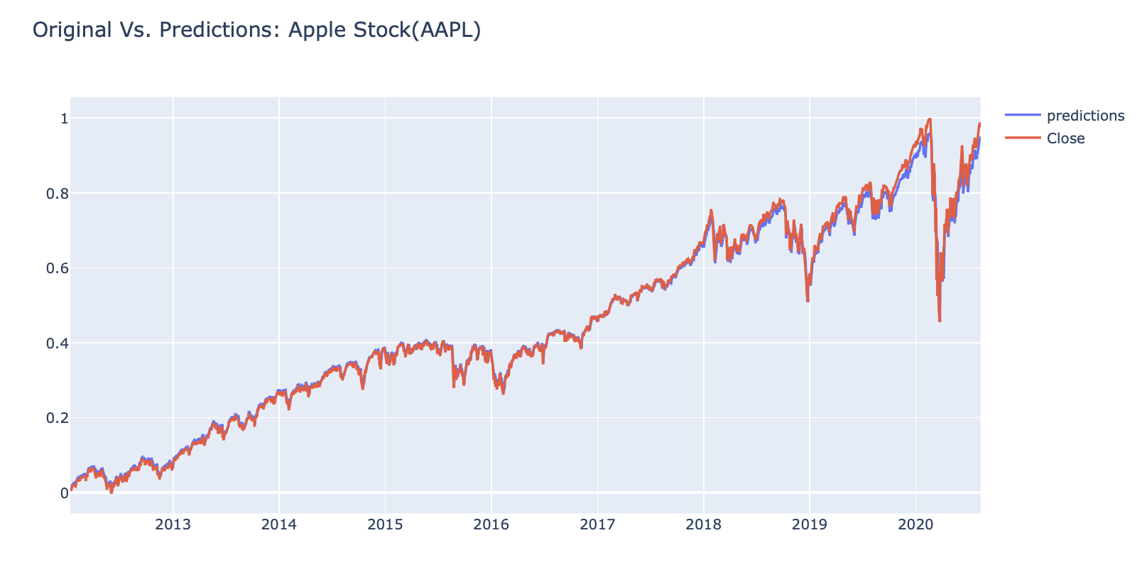
Ridge Regression Score: 0.9311227075637692
# Append the predicted values into a list
predicted_prices = regression_model.predict(X)
predicted = []
for i in predicted_prices:
  predicted.append(i[0])
# Append the close values to the list
close = []
for i in price_volume_target_scaled_df:
  close.append(i[0])
# Create a dataframe based on the dates in the individual stock data
df_predicted = price_volume_target_df[['Date']]
# Add the close values to the dataframe
df_predicted['Close'] = close
# Add the predicted values to the dataframe
df_predicted['Prediction'] = predicted
df_predicted
| Date | Close | Prediction | |
|---|---|---|---|
| 0 | 2012-01-12 | 0.011026 | 0.026286 |
| 1 | 2012-01-13 | 0.010462 | 0.025428 |
| 2 | 2012-01-17 | 0.012209 | 0.026527 |
| 3 | 2012-01-18 | 0.013785 | 0.027022 |
| 4 | 2012-01-19 | 0.013299 | 0.026992 |
| ... | ... | ... | ... |
| 2153 | 2020-08-04 | 0.957606 | 0.866550 |
| 2154 | 2020-08-05 | 0.961583 | 0.871436 |
| 2155 | 2020-08-06 | 1.000000 | 0.903353 |
| 2156 | 2020-08-07 | 0.972088 | 0.878730 |
| 2157 | 2020-08-10 | 0.988245 | 0.892666 |
2158 rows × 3 columns
# Plot the results
#interactive_plot(df_predicted, 'Original Vs. Predictions: Apple Stock(AAPL)')
TRAIN AN LSTM TIME SERIES MODEL
If you want to view APPL / AMZN / ETC: Change ‘sp500 HERE!
# Let's test the functions and get individual stock prices and volumes for sp500
price_volume_df = individual_stock(stocks_df, stocks_vol_df, 'sp500')
# Get the close and volume data as training data (Input)
training_data = price_volume_df.iloc[:, 1:3].values
# Normalize the data
sc = MinMaxScaler(feature_range= (0,1))
training_set_scaled = sc.fit_transform(training_data)
# Create the training and testing data, training data contains present day and previous day values
X = []
y = []
for i in range(1, len(price_volume_df)):
  X.append(training_set_scaled[i-1:i, 0])
  y.append(training_set_scaled[i, 0])
# Convert the data into array format
X = np.array(X)
y = np.array(y)
# Split the data
split = int(0.7 * len(X))
X_train = X[:split]
y_train = y[:split]
X_test = X[split:]
y_test = y[split:]
# Reshape the 1D arrays to 3D arrays to feed in the model
X_train = np.reshape(X_train, (X_train.shape[0], X_train.shape[1], 1))
X_test = np.reshape(X_test, (X_test.shape[0], X_test.shape[1], 1))
# Create the model
inputs = keras.layers.Input(shape=(X_train.shape[1], X_train.shape[2]))
x = keras.layers.LSTM(150, return_sequences= True)(inputs)
x = keras.layers.Dropout(0.3)(x)
x = keras.layers.LSTM(150, return_sequences=True)(x)
x = keras.layers.Dropout(0.3)(x)
x = keras.layers.LSTM(150)(x)
outputs = keras.layers.Dense(1, activation='linear')(x)

model = keras.Model(inputs=inputs, outputs=outputs)
model.compile(optimizer='adam', loss="mse")
model.summary()
Model: "model"
_________________________________________________________________
Layer (type)                 Output Shape              Param #
=================================================================
input_1 (InputLayer)         [(None, 1, 1)]            0
_________________________________________________________________
lstm (LSTM)                  (None, 1, 150)            91200
_________________________________________________________________
dropout (Dropout)            (None, 1, 150)            0
_________________________________________________________________
lstm_1 (LSTM)                (None, 1, 150)            180600
_________________________________________________________________
dropout_1 (Dropout)          (None, 1, 150)            0
_________________________________________________________________
lstm_2 (LSTM)                (None, 150)               180600
_________________________________________________________________
dense (Dense)                (None, 1)                 151
=================================================================
Total params: 452,551
Trainable params: 452,551
Non-trainable params: 0
_________________________________________________________________
# Train the model
history = model.fit(X_train, y_train, epochs= 20, batch_size= 32, validation_split= 0.2)
Epoch 1/20
38/38 [==============================] - 7s 55ms/step - loss: 0.0539 - val_loss: 0.0653
Epoch 2/20
38/38 [==============================] - 0s 8ms/step - loss: 0.0095 - val_loss: 0.0055
Epoch 3/20
38/38 [==============================] - 0s 11ms/step - loss: 0.0012 - val_loss: 5.9507e-04
Epoch 4/20
38/38 [==============================] - 0s 10ms/step - loss: 3.8284e-04 - val_loss: 2.3346e-04
Epoch 5/20
38/38 [==============================] - 0s 9ms/step - loss: 3.5239e-04 - val_loss: 8.1833e-05
Epoch 6/20
38/38 [==============================] - 0s 10ms/step - loss: 3.5036e-04 - val_loss: 6.2046e-05
Epoch 7/20
38/38 [==============================] - 0s 8ms/step - loss: 3.0313e-04 - val_loss: 4.0566e-05
Epoch 8/20
38/38 [==============================] - 0s 9ms/step - loss: 2.8564e-04 - val_loss: 6.2951e-05
Epoch 9/20
38/38 [==============================] - 0s 9ms/step - loss: 3.1342e-04 - val_loss: 5.7098e-05
Epoch 10/20
26/38 [===================>..........] - ETA: 0s - loss: 2.9808e-04
# Make prediction
predicted = model.predict(X)
test_predicted = []

for i in predicted:
  test_predicted.append(i[0])
df_predicted = price_volume_df[1:][['Date']]
df_predicted['predictions'] = test_predicted
close = []
for i in training_set_scaled:
  close.append(i[0])
df_predicted['Close'] = close[1:]
df_predicted
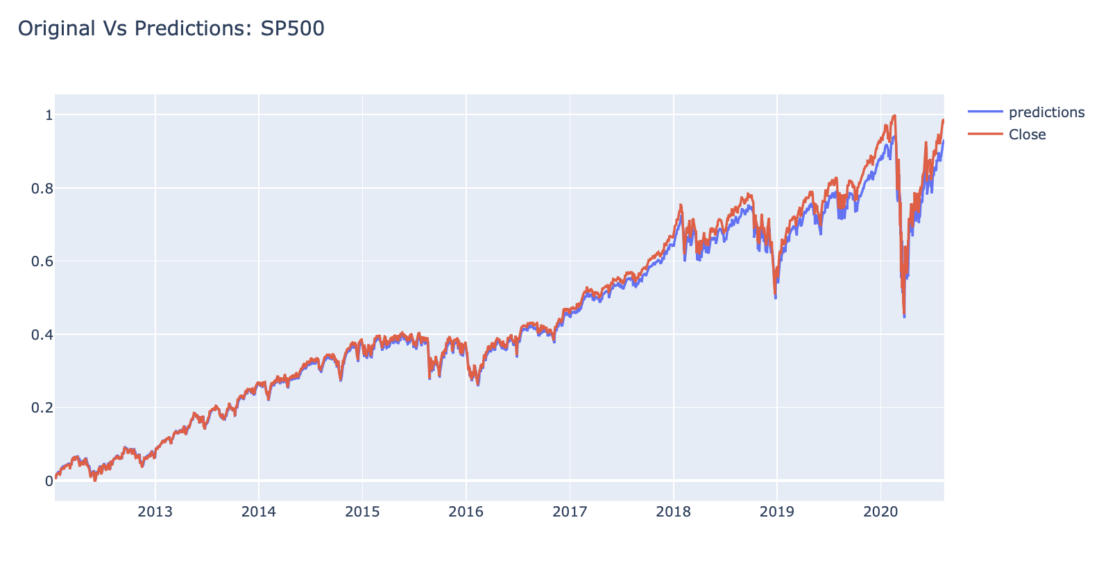
# Plot the results
#interactive_plot(df_predicted, 'Original Vs Predictions: SP500')
Andrew D'Armond
Leveraging data science to achieve results