Wealth of a Nation: Census Income Data

Introduction

The dataset given for this analysis is one from academic purpose to conduct research on a hypothetical census with a focus on the income section. The Y or independant variable of this research will be the X15 variable, which is a reference to the mean income from the total census data. In this case that value was set at 50K. The variable is labeled in the data, which is not shown, as either “1” or “0”. X15 or mean income will have a “1” for a data point if the individual meets the mean income requirements or “0” if the indivual doesn’t.

Research Order

1. Logistic Model Summary
2. Finding of CP value for Decision Tree
3. Decision Tree Model
4. Comparision Curve
5. Conclusion

# Basic Binomial Model and the beginning of our research
library(readr)
census_income <- read_csv("/Users/andrewdarmond/Documents/R/Class 4/census_income.csv")

census_income$X15 <- gsub(">50K", "1", census_income$X15)
census_income$X15 <- gsub("<=50K", "0", census_income$X15)
census_income$X15 <- as.numeric(census_income$X15)

census_logit <- glm(X15~age+capital_gain+capital_lass+hours_per_week+gnlwgt+education_num, data=census_income, family="binomial")
summary(census_logit)

## 
## Call:
## glm(formula = X15 ~ age + capital_gain + capital_lass + hours_per_week + 
##     gnlwgt + education_num, family = "binomial", data = census_income)
## 
## Deviance Residuals: 
##     Min       1Q   Median       3Q      Max  
## -5.3254  -0.6388  -0.4089  -0.1308   3.0998  
## 
## Coefficients:
##                  Estimate Std. Error z value Pr(>|z|)    
## (Intercept)    -8.450e+00  1.207e-01 -70.012  < 2e-16 ***
## age             4.338e-02  1.226e-03  35.372  < 2e-16 ***
## capital_gain    3.186e-04  9.688e-06  32.886  < 2e-16 ***
## capital_lass    7.006e-04  3.258e-05  21.503  < 2e-16 ***
## hours_per_week  4.091e-02  1.325e-03  30.866  < 2e-16 ***
## gnlwgt          5.714e-07  1.477e-07   3.867  0.00011 ***
## education_num   3.232e-01  6.816e-03  47.422  < 2e-16 ***
## ---
## Signif. codes:  0 '***' 0.001 '**' 0.01 '*' 0.05 '.' 0.1 ' ' 1
## 
## (Dispersion parameter for binomial family taken to be 1)
## 
##     Null deviance: 35948  on 32560  degrees of freedom
## Residual deviance: 26472  on 32554  degrees of freedom
## AIC: 26486
## 
## Number of Fisher Scoring iterations: 7

Logistic Model

All variables have the same P value other than gnlwgt. This should indicate the variable is either at the lowest level or in the leaves section of the Decision Tree or won’t be in the model at all. The model shows that all variables have major significance to the model. The AIC is fairly high meaning that the model is not sound as one would hope also. We will drill deeper with the Decision tree model in order find better insights

Next, A CP Tree will be created to determine the proper length for a Decsion Tree Model.

# This will show the best length for our Decision Tree
library(rpart)
library(rpart.plot)
my_tree_cen <- rpart(X15~age+capital_gain+capital_lass+hours_per_week+gnlwgt+education_num, data=census_income, method="class")
#plotcp(my_tree_cen)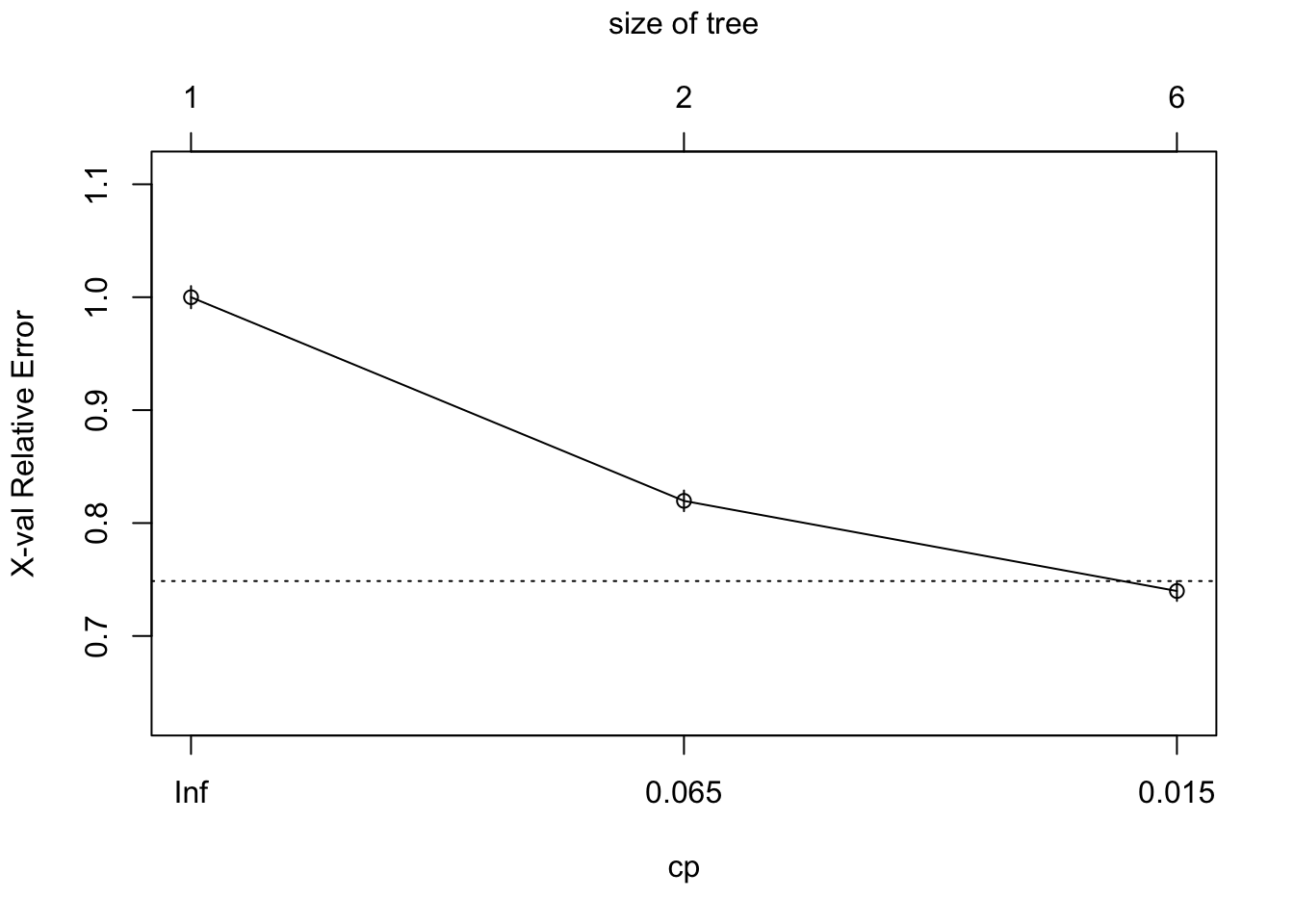

CP Tree

As you can the best value for our cp in the decision tree is set at 0.015. This will create the maximum effectiveness for our decsion tree model. A CP Tree must be found initally before a full Decision Tree is created.

Next, A Decision Tree will be shown in order to illustrate the most influential splitting variables for the data.

# Decision Tree that will show us our most influential variables
library(rpart)
library(rpart.plot)
my_tree_cen <- rpart(X15~age+capital_gain+capital_lass+hours_per_week+gnlwgt+education_num, data=census_income, method="class", cp=0.015)
#rpart.plot(my_tree_cen, extra=1, type=1)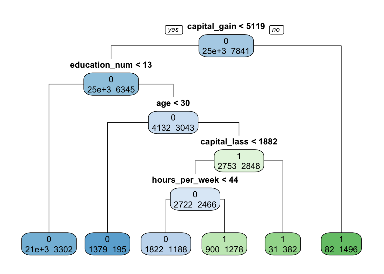

Decision Tree

The two most significant variables are capital gain and education number. Also, since all other variables have the same P value the tree has been split based on which variable has the highest Std. Error in the logistic to the Decision Tree model. The final total of the data leaves is 6. Normally, 6-8 leaves is standard for the Tree so we can infer that our CP is valid. The majority of the data split in the tree is that of individuals with capital gain below 5119 and education under 13 at just over 21000 records all of which fall below the mean income of 50K.

Comparision of Decision Tree and Logistic Model

gnlwgt is the only variable not in the tree, therefore we can decipher that it has the lowest impact among the variables listed in the logistic. This confirms the expectations after the logistic summary. When further comparing the models the next insight gathered would be that the tree was split initially by the variables largest Std. Error, since the P values were all identical as capital gain had the second highest Std. Error behind gnlwgt.

Next, A Comparision Curve will be created to compare the models.

# Creating the comparision curve to fully identify the better model to further our business insights
library(ROCR)
logit_predit_cen <- predict(census_logit, data=census_income, type="response")
val_1_cen <- predict(my_tree_cen, data=census_income, type="prob")
pred_val_cen <- prediction(val_1_cen[,2], census_income$X15)
pred_val_logit_cen <- prediction(logit_predit_cen, census_income$X15)
# Creating the perfromance metric at a true positive to false positive rate
cen_pref <- performance(pred_val_cen, "tpr", "fpr")
cen_pref_logit <- performance(pred_val_logit_cen, "tpr", "fpr")
# Plotting the Curves
#plot(cen_pref, col= "black")
#plot(cen_pref_logit, col= "blue", add=T)
#legend("bottomright", c("Decision Tree", "Logistic Model"), fill= c("black", "blue"))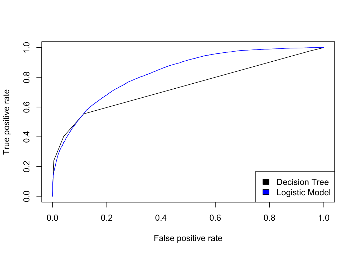

Conclusions

The logistic is the more favorable model. Giving us the better insights when conducting research about data that is centered around the mean income variable or X15 in our census income data.

When the capital gain is less than 5,119 the odds of a person with income under 50K is 99.97%. Additionally, if the person has an education number under 13 then the odds of the person having an income above 50K is 38%.

Finally, We have determined that that if an indiviudal has a higher education with high capital gains then the indivual is the most likely to have an income over the mean of the census. Also that the majority fall under the mean income of 50K.

Source

Hult International Business School